The last time I wrote, I was talking about how spoiled I am by my students. I have two students who did an enormous amount of thinking about a random walk problem I proposed. Just for your reference, the problem was
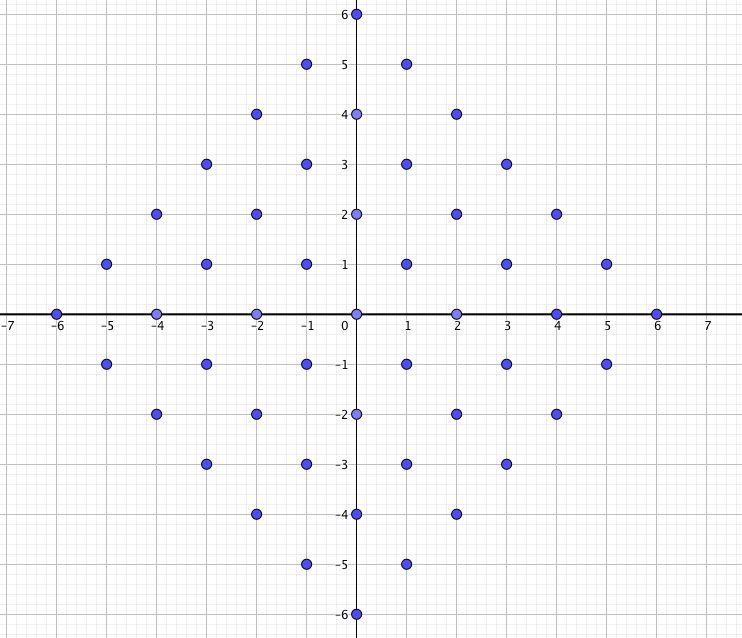
Starting at the origin, a bug jumps one unit either left, right, up, or down. He jumps once each second. List the possible locations (and probabilities associated with those locations) that the bug could be after 6 seconds.
After working on it for awhile with one of my students I waived this one off and told my students to feel free to ignore it. A number did not. Two in particular, Bobby and Matthew (both of whom seemed happy to have me name them!) collaborated over a chat line of some sort and delivered a lovely presentation on their work. I asked them to guest post for me and below is their post. I cannot emphasize enough how impressed I am by their ingenuity and determination. There are two other files they asked me to make available. A 3d representation and a 4d representation generated by their code.
Bobby: Last week, a blog post referred to a random walk problem that our Calculus class worked on, and two students that took a coding approach. We are those two students, and we’re here to discuss how we solved the problem, and the far more interesting work that came after it. For those of you who don’t know, the problem was a 2-dimensional random walk of 6 steps.
Matthew: When I first looked at this problem in class, I thought it would give way far more easily than it actually did. My first attempt was to rewrite the problem as choosing from the four cardinal directions a set of six steps, e.g. {↑ ,→, ↓, ←,←,↓}. By doing so, my hope was to reduce every position on the grid into a set of the bare minimum moves needed to reach it, and pairs of blank spaces which I could fill with a pairs of steps which added to the zero vector. Since the grid had 8-fold symmetry, I was unafraid of solving each point individually, however when the time came to actually do the problem, I found a number of oversights in my initial work which resulted in some pesky double counting.
Bobby: For lazy Calculus students (read: myself), the obvious solution for any random walk problem is to make a computer do it, so i set out to approximate probabilities by running a billion trials of a random walk and counting up the results.
However, this brutish method is relatively unsatisfying, and by the time I finished, Matthew had abandoned his set permutation approach and decided to make a program that iterated through each possible set of 6 steps once and counted up the destinations. This clearly being the better approach, I did the same thing, and we exchanged our results (which matched) and exchanged our code to make improvements: I took some of Matthew’s ideas to make the program easier to scale up and down, and I’d like to think he took some of my ideas and stopped naming variables “DONK,” but I’m sure he didn’t.

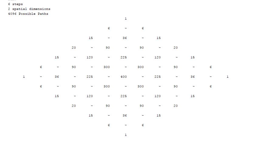
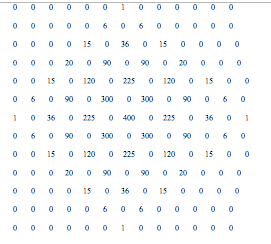
This grid shows the number of ways to land at any given point. After a short time looking over our grid of results, we noticed that each edge of the square was the 6th row of pascal’s triangle. A little more poking around and Matthew noticed that the grid was in fact a multiplication table of that row of the triangle with itself, meaning every entry could be written in the form (nCa)*(nCb), with n being the number of steps and a and b being the relative coordinates of the entry in the table. Finally, we made the observation that this is the 6th layer of Pascal’s square pyramid, a 3d structure much like the triangle where each number is the sum of the four above it. Recalling that a 1d random walk is the nth row of Pascal’s triangle where n = # of steps, a pattern seemed to emerge that we hoped might scale up in dimensions.
Bobby: We did a lot more work, particularly in 3 and 4 dimensions. Our program logic started by defining a variable to track which number walk we were on, and keyed in on the base-four version of that number to define a set of moves for our bug. For example, test 5 translates to 000011 in base 4, and the bug reads each digit individually, right to left, using it as an instruction for motion: 0 = right, 1 = up, 2 = left, 3 = down, translating 000011 to U, U, R, R, R, R.
This logic makes it easy to change the number of dimensions or steps, so we went to 3 dimensions, expecting to get 3-dimensional cross-sections of some 4-dimensional solid for each particular solution. The results did not disappoint, as we got the expected octahedron as a result. Obviously, this output was a little tough to format, but I think what we settled on is easy enough to read. Each grid separated by the others from a row of asterisks is a 2d cross-section of the solution octahedron. LINK DATA Stack those layers on top of each other and the visualization is pretty easy, I think.
At this point, we had to do four dimensions, and had a good idea of how it would look. The 2d solution is the shape of the 1d solution stacked on itself, the 3d solution is a stack of the shapes of the 2d solution, so we the 4d solution would obviously be a series of 3d octahedrons in the same x, y, z, but translated along our fourth spatial axis. It took me a moment to wrap my head around this data, but I’ve become very comfortable with it. LINK DATA Each section under the rows reading “NEW 3D SOLID…” is a series of grids that are stacked into an octahedron, and then the octahedrons are stacked on each other in the fourth spatial dimension. This, of course, is also a 4d cross-section of a 5d Pascalian solid, each nth 4d layer of which is a solution to the 4d random walk of n steps, but that’s about as far as I can go envisioning these shapes. Matthew tells me the 5d structure is “Pascal’s Orthoplexal Hyperpyramid” but I’m not sure I can trust that.
Matthew: Of course, the idea of layers of Pascal’s square pyramid as multiplication tables of the rows of Pascal’s triangle is a fascinating one, and one I sought to prove. Though my initial effort to prove it algebraically did meet with success, I was unsatisfied with my clunky proof and did some quick googling on the subject. My search turned up a blog with a simple proof by induction, far more elegant than anything I had done. Still, I find that proofs by induction are rarely enough to understand a result intuitively, and so I continued working with Bobby, looking for a better way to interpret the formula in terms of the problem, as well as potentially a way of generalizing the result to higher dimensional walks.
Eventually, I took a step back from the symbol soup and searched for a more intuitive interpretation of the formula we had discovered in terms of the original problem. After some while, I had an epiphany while placing the problem back into the language of sets. My initial idea of viewing the problem as selecting a set of 6 steps along cardinal directions could be reformulated in a way which made the formula obvious. Instead of considering steps along the cardinal directions like the original problem had stated, I realized that every unit vector along a cardinal direction could be rewritten uniquely as the sum of two diagonal vectors of magnitude √2/2, e.g. {↑} = {↖,↗}. With this realization in hand, the original problem can be rephrased as a random walk in six steps of magnitude √2/2 along the line y=x, followed by another random walk of six steps perpendicular to the first. Or, to give an example in my initial interpretation of the problem as sets of steps, the two dimensional walk {↑ ,→, ↓, ←,←,↓} is the same walk as {{↖,↗},{↘,↗},{↘,↙},{↖,↙},{↖,↙},{↘,↙}}, which is the same as the union of the two one dimensional walks {↖,↘,↘,↖,↖,↘} and {↗,↗,↙,↙,↙,↙}. Once the problem is reformulated in this way, the reason why the table obeys such a simple multiplicative relationship in two dimensions becomes satisfyingly clear. Though I am pleased that we were able to transform such an originally dense and unapproachable problem into a setting where it is obvious, we have unfortunately as of yet been unable to find an application of this method to higher dimensions.


